The data build tool (dbt) is an effective data transformation tool and it supports key AWS analytics services – Redshift, Glue, EMR and Athena. In part 1 of the dbt on AWS series, we discuss data transformation pipelines using dbt on Redshift Serverless. Subsets of IMDb data are used as source and data models are developed in multiple layers according to the dbt best practices.
Part 1 – Redshift (this post)
Motivation
In our experience delivering data solutions for our customers, we have observed a desire to move away from a centralised team function, responsible for the data collection, analysis and reporting, towards shifting this responsibility to an organisation’s lines of business (LOB) teams. The key driver for this comes from the recognition that LOBs retain the deep data knowledge and business understanding for their respective data domain; which improves the speed with which these teams can develop data solutions and gain customer insights. This shift away from centralised data engineering to LOBs exposed a skills and tooling gap.
Let’s assume as a starting point that the central data engineering team has chosen a project that migrates an on-premise data warehouse into a data lake (spark + iceberg + redshift) on AWS, to provide a cost-effective way to serve data consumers thanks to iceberg’s ACID transaction features. The LOB data engineers are new to spark and they have a little bit of experience in python while the majority of their work is based on SQL. Thanks to their expertise in SQL, however, they are able to get started building data transformation logic on jupyter notebooks using pyspark. However they soon find the codebase gets quite bigger even during the minimum valuable product (MVP) phase, which would only amplify the issue as they extend it to cover the entire data warehouse. Additionally the use of notebooks makes development challenging mainly due to lack of modularity and failing to incorporate testing. Upon contacting the central data engineering team for assistance they are advised that the team uses scala and many other tools (e.g. Metorikku) that are successful for them, however cannot be used directly by the engineers of the LOB. Moreover the engineering team don’t even have a suitable data transformation framework that supports iceberg. The LOB data engineering team understand that the data democratisation plan of the enterprise can be more effective if there is a tool or framework that:
-
can be shared across LOBs although they can have different technology stack and practices,
-
fits into various project types from traditional data warehousing to data lakehouse projects, and
-
supports more than a notebook environment by facilitating code modularity and incorporating testing.
The data build tool (dbt) is an open-source command line tool and it does the T in ELT (Extract, Load, Transform) processes well. It supports a wide range of data platforms and the following key AWS analytics services are covered – Redshift, Glue, EMR and Athena. It is one of the most popular tools in the modern data stack that originally covers data warehousing projects. Its scope is extended to data lake projects by the addition of the dbt-spark and dbt-glue adapter where we can develop data lakes with spark SQL. Recently the spark adapter added open source table formats (hudi, iceberg and delta lake) as the supported file formats and it allows you to work on data lake house projects with it. As discussed in this blog post, dbt has clear advantages compared to spark in terms of
-
low learning curve as SQL is easier than spark
-
better code organisation as there is no correct way of organising transformation pipeline with spark
On the other hand, its weaknesses are
-
lack of expressiveness as Jinja is quite heavy and verbose, not very readable, and unit-testing is rather tedious
-
limitation of SQL as some logic is much easier to implement with user defined functions rather than SQL
Those weaknesses can be overcome by Python models as it allows you to apply transformations as DataFrame operations. Unfortunately the beta feature is not available on any of the AWS services, however it is available on Snowflake, Databricks and BigQuery. Hopefully we can use this feature on Redshift, Glue and EMR in the near future.
Finally the following areas are supported by spark, however not supported by DBT:
-
E and L of ELT processes
-
real time data processing
Overall dbt can be used as an effective tool for data transformation in a wide range of data projects from data warehousing to data lake to data lakehouse. Also it can be more powerful with spark by its Python models feature. Below shows an overview diagram of the scope of this dbt on AWS series. Redshift is highlighted as it is discussed in this post.

Infrastructure
A VPC with 3 public and private subnets is created using the AWS VPC Terraform module. The following Redshift serverless resources are deployed to work with the dbt project. As explained in the Redshift user guide, a namespace is a collection of database objects and users and a workgroup is a collection of compute resources. We also need a Redshift-managed VPC endpoint for a private connection from a client tool. The source can be found in the GitHub repository of this post.
# redshift-sls/infra/redshift-sls.tf |
As in the previous post, we connect to Redshift via SoftEther VPN to improve developer experience significantly by accessing the database directly from the developer machine. Instead of providing VPN related secrets as Terraform variables in the earlier post, they are created internally and stored to AWS Secrets Manager. Also the Redshift admin username and password are included so that the secrets can be accessed securely. The details can be found in redshift-sls/infra/secrets.tf and the secret string can be retrieved as shown below.
$ aws secretsmanager get-secret-value –secret-id redshift-sls-all-secrets –query “SecretString” –output text |
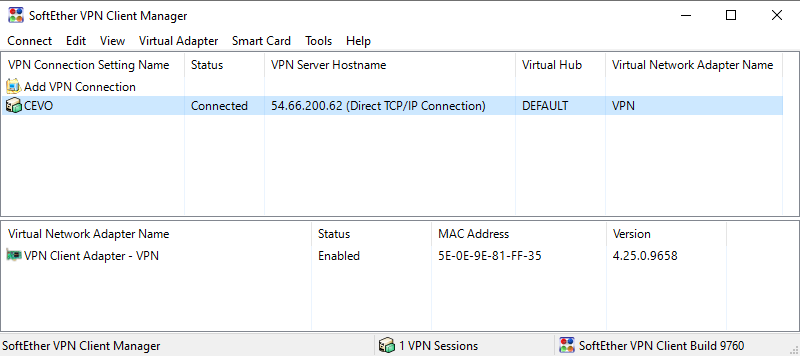
The previous post demonstrates how to create a VPN user and to establish connection in detail. An example of a successful connection is shown below.
Project
We build a data transformation pipeline using subsets of IMDb data – seven titles and names related datasets are provided as gzipped, tab-separated-values (TSV) formatted files. This results in three tables that can be used for reporting and analysis.
Create Database Objects
The majority of data transformation is performed in the imdb schema, which is configured as the dbt target schema. We create the final three tables in a custom schema named imdb_analytics. Note that its name is according to the naming convention of the dbt custom schema, which is <target_schema>_<custom_schema>. After creating the database schemas, we create a development user (dbt) and a group that the user belongs to, followed by granting necessary permissions of the new schemas to the new group and reassigning schema ownership to the new user.
— redshift-sls/setup-redshift.sql — // create db schemas |
Save Data to S3
The Axel download accelerator is used to download the data files locally followed by decompressing with the gzip utility. Note that simple retry logic is added as I see download failure from time to time. Finally the decompressed files are saved into the project S3 bucket using the S3 sync command.
# redshift-sls/upload-data.sh #!/usr/bin/env bash while true; |
Copy Data
The data files in S3 are loaded into Redshift using the COPY command as shown below.
— redshift-sls/setup-redshift.sql — // copy data to tables |
Initialise dbt Project
We need the dbt-core and dbt-redshift. Once installed, we can initialise a dbt project with the dbt init command. We are required to specify project details such as project name, database adapter and database connection info. Note dbt creates the project profile to .dbt/profile.yml of the user home directory by default.
$ dbt init |
dbt initialises a project in a folder that matches to the project name and generates project boilerplate as shown below. Some of the main objects are dbt_project.yml, and the model folder. The former is required because dbt doesn’t know if a folder is a dbt project without it. Also it contains information that tells dbt how to operate on the project. The latter is for including dbt models, which is basically a set of SQL select statements. See dbt documentation for more details.
$ tree dbt_redshift_sls/ -L 1 |
We can check the database connection with the dbt debug command. Do not forget to connect to VPN as mentioned earlier.
$ dbt debug |
After initialisation, the model configuration is updated. The project materialisation is specified as view although it is the default materialisation. Also tags are added to the entire model folder as well as folders of specific layers – staging, intermediate and marts. As shown below, tags can simplify model execution.
# redshift-sls/dbt_redshift_sls/dbt_project.yml …
|
Two dbt packages are used in this project. The dbt-labs/codegen is used to save typing when generating the source and base models while dbt-labda/dbt_utils for adding tests to the final marts models. The packages can be installed by the dbt deps command.
# redshift-sls/dbt_redshift_sls/packages.yml |
Create dbt Models
The models for this post are organised into three layers according to the dbt best practices – staging, intermediate and marts.
Staging
The seven tables that are loaded from S3 are dbt source tables and their details are declared in a YAML file (_imdb_sources.yml). By doing so, we are able to refer to the source tables with the {{ source() }} function. Also we can add tests to source tables. For example below two tests (unique, not_null) are added to the tconst column of the title_basics table below and these tests can be executed by the dbt test command.
# redshift-sls/dbt_redshift_sls/models/staging/imdb/_imdb__sources.yml |
Based on the source tables, staging models are created. They are created as views, which is the project’s default materialisation. In the SQL statements, column names and data types are modified mainly.
— // redshift-sls/dbt_redshift_sls/models/staging/imdb/stg_imdb__title_basics.sql |
Below shows the file tree of the staging models. The staging models can be executed using the dbt run command. As we’ve added tags to the staging layer models, we can limit to execute only this layer by dbt run –select staging.
redshift-sls/dbt_redshift_sls/models/staging/ |
Intermediate
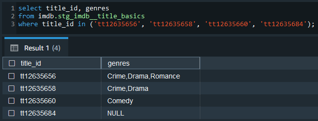
We can keep intermediate results in this layer so that the models of the final marts layer can be simplified. The source data includes columns where array values are kept as comma separated strings. For example, the genres column of the stg_imdb__title_basics model includes up to 3 genre values as shown below.
A total of seven columns in three models are columns of comma-separated strings and it is better to flatten them in the intermediate layer. Also, in order to avoid repetition, a dbt macro (flatten_fields) is created to share the column-flattening logic.
# redshift-sls/dbt_redshift_sls/macros/flatten_fields.sql |
The macro function can be added inside a recursive cte by specifying the relevant model, field name to flatten and id field name.
— dbt_redshift_sls/models/intermediate/title/int_genres_flattened_from_title_basics.sql with recursive cte (id, idx, field) as ( |
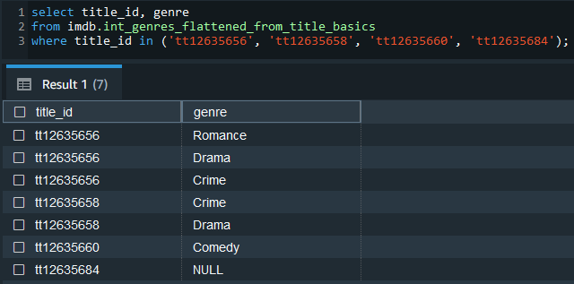
The intermediate models are also materialised as views and we can check the array columns are flattened as expected.
Below shows the file tree of the intermediate models. Similar to the staging models, the intermediate models can be executed by dbt run –select intermediate.
redshift-sls/dbt_redshift_sls/models/intermediate/ |
Marts
The models in the marts layer are configured to be materialised as tables in a custom schema. Their materialisation is set to table and the custom schema is specified as analytics. Note that the custom schema name becomes imdb_analytics according to the naming convention of dbt custom schemas. Models of both the staging and intermediate layers are used to create final models to be used for reporting and analytics.
— redshift-sls/dbt_redshift_sls/models/marts/analytics/titles.sql |
The details of the three models can be found in a YAML file (_analytics__models.yml). We can add tests to models and below we see tests of row count matching to their corresponding staging models.
# redshift-sls/dbt_redshift_sls/models/marts/analytics/_analytics__models.yml |
Below shows the file tree of the marts models. As with the other layers, the marts models can be executed by dbt run –select marts.
redshift-sls/dbt_redshift_sls/models/marts/ |
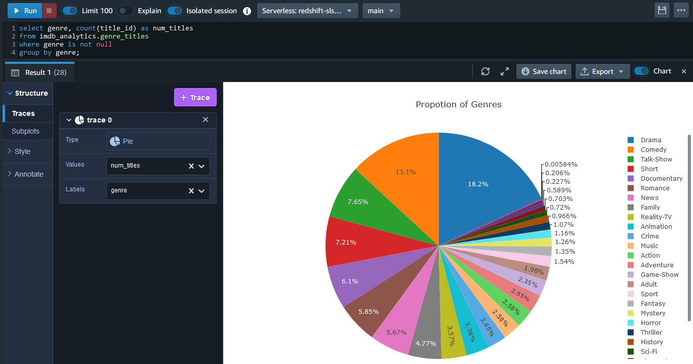
Using the Redshift query editor v2, we can quickly create charts with the final models. The example below shows a pie chart and we see about 50% of titles are from the top 5 genres.
Generate dbt Documentation
A nice feature of dbt is documentation. It provides information about the project and the data warehouse and it facilitates consumers as well as other developers to discover and understand the datasets better. We can generate the project documents and start a document server as shown below.
$ dbt docs generate |
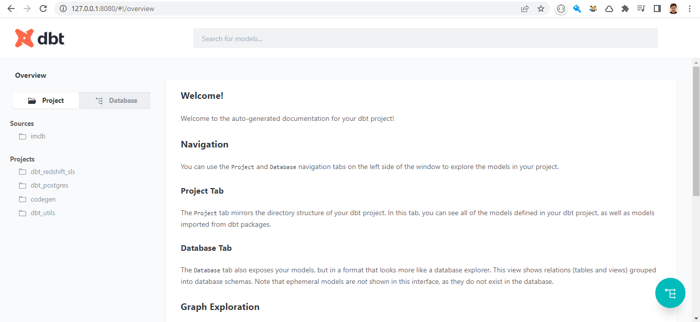
A very useful element of dbt documentation is data lineage, which provides an overall view about how data is transformed and consumed. Below we can see that the final titles model consumes all title-related stating models and an intermediate model from the name basics staging model.

Summary
In this post, we discussed how to build data transformation pipelines using dbt on Redshift Serverless. Subsets of IMDb data are used as source and data models are developed in multiple layers according to the dbt best practices. dbt can be used as an effective tool for data transformation in a wide range of data projects from data warehousing to data lake to data lakehouse and it supports key AWS analytics services – Redshift, Glue, EMR and Athena. More examples of using dbt will be discussed in subsequent posts.

